Robot Kinematics Explained: The Mathematical Engine of CNC Automation
The Geometry of Motion: Unlocking Robotic Precision
In the world of high-precision CNC machining, where the path of a cutting tool defines the quality and accuracy of a final component, understanding motion is paramount. For industrial robots, the science that governs this motion is robot kinematics. This is not merely a theoretical discipline confined to academic papers; it is the fundamental mathematical engine that translates a digital command in a control program into the precise, coordinated movement of a robotic arm in three-dimensional space. For an advanced manufacturing partner like JLYPT, where we integrate robotic automation with 5-axis milling and EDM processes, a deep, practical understanding of robot kinematics explained is what separates a functional automated cell from an optimized, high-performance production asset.
At its core, kinematics is the study of motion without considering the forces that cause it. In robotics, it provides the essential framework for answering two critical questions: 1) Given a set of joint angles, where is the robot’s tool? (Forward Kinematics). 2) To place the tool at a desired position and orientation, what joint angles are required? (Inverse Kinematics). Mastering these questions is the key to programming complex paths, avoiding collisions, and achieving the micron-level repeatability demanded in machining environments. This comprehensive guide will demystify robot kinematics explained, moving from foundational mathematical concepts to their direct application in CNC machining tasks like complex contouring, multi-machine tending, and adaptive finishing.
Part 1: The Foundational Language of Kinematics
To understand how a robot moves, we must first define the language used to describe its structure and position.
1.1 Links, Joints, and Degrees of Freedom (DoF)
A robotic arm is a chain of rigid bodies called links, connected by movable joints.
-
Links: The structural elements, such as the base, upper arm, forearm, and wrist segments. Their lengths and shapes define the robot’s physical reach and work envelope.
-
Joints: The articulations that allow relative motion between links. In industrial robots, these are almost exclusively revolute joints (rotational) or, less commonly, prismatic joints (linear slides). A standard 6-axis articulated robot has six revolute joints.
-
Degrees of Freedom (DoF): Each independent joint provides one degree of freedom. Six DoF are typically required to arbitrarily position and orient a tool in 3D space (three for X, Y, Z position; three for roll, pitch, yaw orientation).
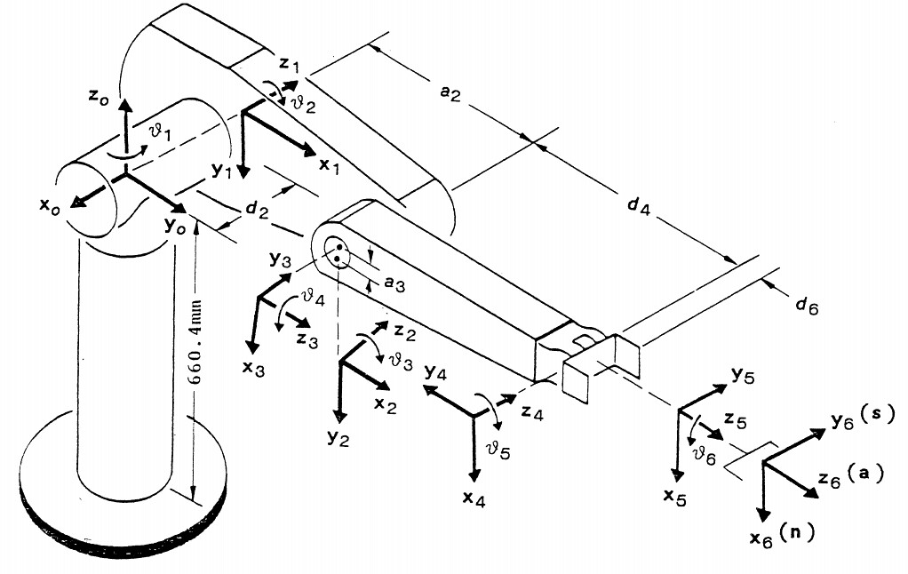
1.2 Coordinate Frames and Transformations
The position of anything in space is always described relative to a reference point. In robotics, we attach coordinate frames (an origin and X, Y, Z axes) to each link.
-
Base Frame (Frame {0}): Fixed to the robot’s stationary base. The world coordinate system.
-
Tool Center Point (TCP) Frame (Frame {TCP}): Attached to the robot’s end-effector or tool. This is the frame we ultimately control—the point we want to move along a specific path, like a deburring tool following a part edge.
-
Homogeneous Transformation Matrices: The mathematical magic that connects these frames. A 4×4 transformation matrix
Tdescribes the position and orientation of one coordinate frame relative to another. It combines rotation and translation into a single, computable entity. The chain of transformations from the base to the TCP is the heart of kinematic modeling.
Part 2: Forward Kinematics – Predicting the Tool’s Pose
Forward Kinematics (FK) is the straightforward calculation: given the measured angle of every joint in the robot (θ₁, θ₂, …, θ₆), compute the precise position and orientation (collectively called the pose) of the TCP.
2.1 The Denavit-Hartenberg (D-H) Convention
To systematically derive the kinematic equations for any serial-link robot, the Denavit-Hartenberg (D-H) parameters convention is used. It’s a standardized method to assign coordinate frames to each link using just four parameters per joint:
-
Link Length (a): The distance along one link’s X-axis to the next joint.
-
Link Twist (α): The twist angle between one link’s Z-axis and the next link’s Z-axis.
-
Link Offset (d): The distance along one joint’s Z-axis to the next link.
-
Joint Angle (θ): The rotation angle about the joint’s Z-axis (the variable for revolute joints).
For a 6-axis robot, this gives us a table of 4 x 6 = 24 parameters that completely describe its geometric structure.
2.2 The Forward Kinematics Equation
Using the D-H parameters, we can construct the homogeneous transformation matrix for each link-to-link movement. The overall transformation from the base frame {0} to the tool frame {TCP} is found by multiplying these individual matrices together in sequence:
T_base_tool = A₁(θ₁) * A₂(θ₂) * A₃(θ₃) * A₄(θ₄) * A₅(θ₅) * A₆(θ₆)
This single 4×4 matrix, T_base_tool, contains all the information: its upper-left 3×3 sub-matrix defines the tool’s orientation, and its rightmost 3×1 column vector defines the tool’s X, Y, Z coordinates in the base frame. Every modern robot controller has this FK model built-in, constantly calculating the TCP pose for display, monitoring, and as the first step in more complex control loops.
Table 1: The Four Denavit-Hartenberg (D-H) Parameters
| Parameter | Symbol | Description | Role in Kinematic Model |
|---|---|---|---|
| Link Length | a |
The perpendicular distance between the Z-axes of two successive joints. | Defines the physical length of the link between joint rotation axes. |
| Link Twist | α |
The angle between the Z-axes of two successive joints, measured about their common normal (X-axis). | Accounts for any “twist” or non-parallel alignment between adjacent joint axes. |
| Link Offset | d |
The distance along the Z-axis of a joint from one link to the next. | Represents the offset along a joint’s axis before the next link begins (common in shoulder/elbow/wrist designs). |
| Joint Angle | θ |
The angle of rotation about the joint’s Z-axis between one link and the next. | The primary variable for a revolute joint. This is the value commanded by the controller to move the robot. |
Part 3: Inverse Kinematics – The Core of Robot Programming
While FK is deterministic, Inverse Kinematics (IK) is the essential, complex problem that makes robotics practical. The question is: given a desired TCP pose (from a CAD path or a taught point), what are the necessary joint angles (θ₁…θ₆) to achieve it?
3.1 The Challenge of Multiple Solutions
For a 6-axis robot arm, the IK problem is nonlinear and often has multiple valid solutions—a concept known as kinematic redundancy for the same TCP pose.
-
Lefty/Righty Configuration: The elbow can be to the left or right of the line connecting shoulder to wrist.
-
Elbow Up/Elbow Down: The elbow joint can be above or below the shoulder-wrist plane.
-
Wrist Flip: The wrist joints can often achieve the same tool orientation in two different ways.
The robot controller’s IK solver must choose one solution based on criteria like:
-
Minimal joint movement from the current position.
-
Avoidance of singularities (positions where the robot loses a degree of freedom).
-
Maintaining a “preferred” configuration (e.g., always elbow-up) for consistency.
3.2 Solving Methods
-
Analytical/Closed-Form Solution: For robots with certain kinematic designs (like spherical wrists), the IK equations can be solved directly using trigonometric identities. This is fast and deterministic, used by most industrial robot controllers.
-
Numerical Solution: For more complex or redundant arms, iterative numerical methods (like the Jacobian-based gradient descent) are used. The solver makes an initial guess and iteratively adjusts the joint angles until the calculated TCP pose is sufficiently close to the target.
Table 2: Forward vs. Inverse Kinematics in Robotic CNC Applications
| Aspect | Forward Kinematics (FK) | Inverse Kinematics (IK) |
|---|---|---|
| Core Question | Where is the tool given the joint angles? | What joint angles are needed to place the tool here? |
| Input | Set of all joint angles (θ₁…θ₆). | Desired Tool Center Point (TCP) position and orientation (6D pose). |
| Output | TCP position (X, Y, Z) and orientation (Roll, Pitch, Yaw). | Set of all joint angles (θ₁…θ₆). |
| Computational Complexity | Relatively simple, deterministic matrix multiplication. | Complex, often non-linear. May have multiple or no solutions. |
| Primary Role in Control | Used for monitoring, simulation, and as the first step in sensor-based control loops. | The fundamental enabler of programming. Every move command (MoveL, MoveJ) requires an IK solution. |
| Example in CNC Machining | The control system displays the live position of a deburring tool overlaid on a part drawing. | Programming a robot to follow a 5-axis toolpath extracted from a CAM system for milling a complex mold. |
Part 4: Advanced Kinematic Concepts in Precision Machining
Beyond basic FK/IK, several advanced kinematic concepts are critical for deploying robots in high-accuracy CNC environments.
4.1 Singularities and Their Impact
A kinematic singularity is a specific joint configuration where the robot loses one or more degrees of freedom. In these poses, the Jacobian matrix (which maps joint velocities to TCP velocities) becomes rank-deficient.
-
Types: Common singularities include wrist singularity (axes 4 and 6 align), elbow singularity (the arm is fully extended or retracted), and shoulder singularity.
-
Consequences: Near a singularity, tiny movements in Cartesian space (TCP) require extremely large, rapid movements in joint space. This can cause:
-
Loss of Control: The controller cannot execute the commanded Cartesian path.
-
Extreme Joint Speeds: Risk of exceeding motor or reducer limits.
-
Path Deviation: The robot may deviate from the programmed path to avoid the singularity.
-
-
Mitigation: Advanced offline programming (OLP) software simulates and automatically modifies paths to avoid singular configurations, ensuring smooth, executable programs for complex contouring operations.
4.2 The Tool Center Point (TCP) and Work Object Frames
A robot’s kinematic chain doesn’t end at its flange. The Tool Center Point (TCP) is a user-defined point on the tool (e.g., the tip of a drill, the center of a gripper).
-
TCP Definition: The position and orientation of the TCP relative to the robot’s flange is defined by a transformation matrix. Accurate TCP calibration (using methods like the 4-point or 6-point method) is absolutely critical for any precision task. An error of 0.1mm in TCP definition becomes a 0.1mm error on the part.
-
Work Object Frames: Similarly, the part or fixture is defined by a work object coordinate system. This allows programmers to define paths relative to the part, not the robot base. If the part is moved (on a pallet), only the work object frame needs updating, not the entire program. This is essential for flexible, palletized systems common in machining cells.
4.3 Kinematic Calibration for Accuracy
A robot’s nominal kinematic model (its D-H parameters) is based on ideal drawings. Real-world manufacturing tolerances, assembly errors, and load-induced deflections cause deviations.
-
Process: Kinematic calibration uses an external high-precision measurement system (like a laser tracker) to measure the actual TCP pose at dozens of locations throughout the work volume. Sophisticated software compares these measurements to the poses predicted by the nominal model and calculates corrected D-H parameters.
-
Outcome: This process can improve a robot’s absolute accuracy from several millimeters to within ±0.1 mm or better over its entire workspace. For robotic drilling or machining, where the robot must go to a point defined in an external CAD coordinate system, this is a non-negotiable procedure.
Part 5: Practical Applications in CNC Machining – A Kinematic Perspective
The abstract mathematics of kinematics manifest directly in tangible machining applications.
5.1 Complex 5-Axis Tool Path Execution
When a robot is used for direct milling or trimming (e.g., of composite aerospace parts), it must follow a 5-axis toolpath from a CAM system.
-
Kinematic Role: The toolpath is a sequence of desired TCP poses (position + tool orientation vector). The robot’s controller must solve the IK problem for each pose along the path at a very high rate (hundreds of times per second) to generate smooth joint motions. The choice of kinematic configuration (elbow-up vs. elbow-down) must remain consistent to avoid mid-path flips that would cause a pause or discontinuity. The look-ahead function pre-solves IK for many points ahead to optimize velocity and acceleration.
5.2 Multi-Axis Machine Tending with External Axes
In a cell where one robot tends multiple CNC machines or a large machining center with a pallet system, the robot is often mounted on a linear track (7th axis).
-
Kinematic Role: The linear track becomes an additional prismatic joint in the robot’s kinematic chain. The controller’s kinematic model expands to 7 DoF, creating a more redundant system. The IK solver now has infinite ways to achieve a TCP pose, allowing it to optimize for goals like “keep the arm centered on the track to maximize reach” or “avoid a collision with a specific machine door” while still hitting the target. This is an example of redundancy resolution.
5.3 Force-Guided Adaptive Finishing
In deburring or polishing, a force/torque sensor provides feedback.
-
Kinematic Role: The controller runs a hybrid position/force control loop. The desired path provides the positional trajectory (solved via IK). The force error (desired vs. measured contact force) generates a corrective Cartesian velocity vector. This velocity vector is then fed into the robot’s inverse Jacobian to calculate the required joint velocity corrections. This seamlessly blends kinematic path-following with real-world force interaction, allowing the robot to adapt to part variations.
Part 6: Case Studies: Kinematics in Action
Case Study 1: Robotic Trimming of a Large Composite Aircraft Wing Skin
-
Challenge: Trim the edges and cutouts of a large, curved carbon-fiber wing skin. A 5-axis CNC gantry was too expensive. The robot needed to follow a complex 5-axis path with high stiffness to prevent chatter and delamination.
-
Kinematic Analysis & Solution: The robot was mounted on a long linear track to cover the part’s length, creating a 7-DoF system. First, the entire system underwent volumetric kinematic calibration with a laser tracker to achieve the necessary absolute accuracy. The CAM path defined the TCP (router bit tip) pose relative to the part coordinate system. The robot’s advanced IK solver, aware of the 7th axis, was configured to prioritize a “stiff” configuration—minimizing the extension of J2 and J3—to maximize rigidity during cutting. Singularity avoidance algorithms were tuned to ensure smooth transitions, especially when the wrist needed to reorient for cutting perpendicular to the contoured surface.
-
Outcome: The kinematic configuration and calibration allowed the robotic cell to perform the high-precision trimming operation successfully, holding aerospace tolerances. The redundant axis allowed the cell to optimize its posture continuously for stiffness throughout the large work envelope.
Case Study 2: Flexible Palletized Machining Cell for Engine Blocks
-
Challenge: Machine different V6 and V8 engine blocks on the same horizontal machining center (HMC). A robot needed to load raw castings from various incoming pallets onto the HMC’s pallet changer, then remove finished parts to an outgoing pallet. Part locations on the pallets were not perfectly uniform.
-
Kinematic Analysis & Solution: The system used a 6-axis robot. A 3D vision system located each casting on the inbound pallet. The vision output was a 6D pose (X, Y, Z, R, P, Y) of the casting relative to the camera. Using frame transformations, this pose was converted into the robot’s base coordinate system. This desired “grasp pose” was then fed to the robot’s IK solver. The key here was the precise definition and transformation of multiple coordinate frames: Camera Frame, Pallet Frame, Robot Base Frame, and TCP Frame (custom gripper). Accurate hand-eye calibration was critical to make this transformation chain work. For each engine block type, a different TCP was selected in the program, and the IK solver automatically calculated the appropriate joint angles.
-
Outcome: The cell achieved flexible, untended production. The robust kinematic frame management allowed it to handle part position variation without mechanical fixturing, demonstrating how IK integrates with sensor data for adaptive operation.
Case Study 3: Precision Robotic Drilling for Aerospace Assembly
-
Challenge: Drill hundreds of fastener holes in an aircraft fuselage panel with tight positional tolerances (±0.1mm). The large panel was held in a single, massive fixture.
-
Kinematic Analysis & Solution: A high-accuracy robotic arm was chosen. The drilling path was generated from the CAD model of the panel. To overcome the robot’s inherent lack of absolute accuracy, a metrology-assisted closed-loop system was implemented. An optical tracking system (like laser radar) continuously measured the 3D position of reflective targets on the robot’s arm. This real-world measurement was compared to the robot’s internal FK calculation (based on its joint encoders). The discrepancy was used to create a dynamic error map, and corrections were fed back to the IK solver in real-time. Essentially, the system created a feedback loop around the robot’s entire kinematic chain, using external data to correct for kinematic model errors, thermal drift, and deflection under the drilling thrust force.
-
Outcome: The system achieved the required drilling precision, a feat impossible with the robot’s standard open-loop kinematics. This case represents the cutting-edge integration of kinematic modeling with real-time metrology to push robotic accuracy into the CNC domain.
Conclusion: From Equations to Execution
Robot kinematics explained reveals the elegant mathematical backbone that makes industrial robotics possible. It is the indispensable link between the abstract world of digital programming and the physical world of precise motion. For manufacturers and integrators, a functional grasp of these principles—from the multiplication of transformation matrices to the practical implications of singularities and TCP definition—is crucial for designing, programming, and troubleshooting advanced automated cells.
As robotics continues to converge with high-precision CNC machining, the role of kinematics only grows more central. The future lies in more sophisticated models that account for dynamic deflections, in real-time kinematic calibration, and in smarter IK solvers that can optimize for energy efficiency, tool life, and path quality simultaneously.
At JLYPT, our engineering philosophy is rooted in this deep technical understanding. We recognize that successful automation is built not just on powerful hardware, but on a precise command of the underlying science of motion. By applying the principles of robot kinematics, we ensure that the robotic solutions we integrate or work alongside perform with the precision, reliability, and intelligence demanded by modern manufacturing.
Ready to engineer a robotic solution where every movement is calculated for optimal precision? Contact JLYPT to discuss how a mastery of kinematics and system integration can transform your machining operations. Discover our approach to precision-engineered automation at JLYPT CNC Machining Services.